Beyond a Single Best Fit: Probabilistic History Matching

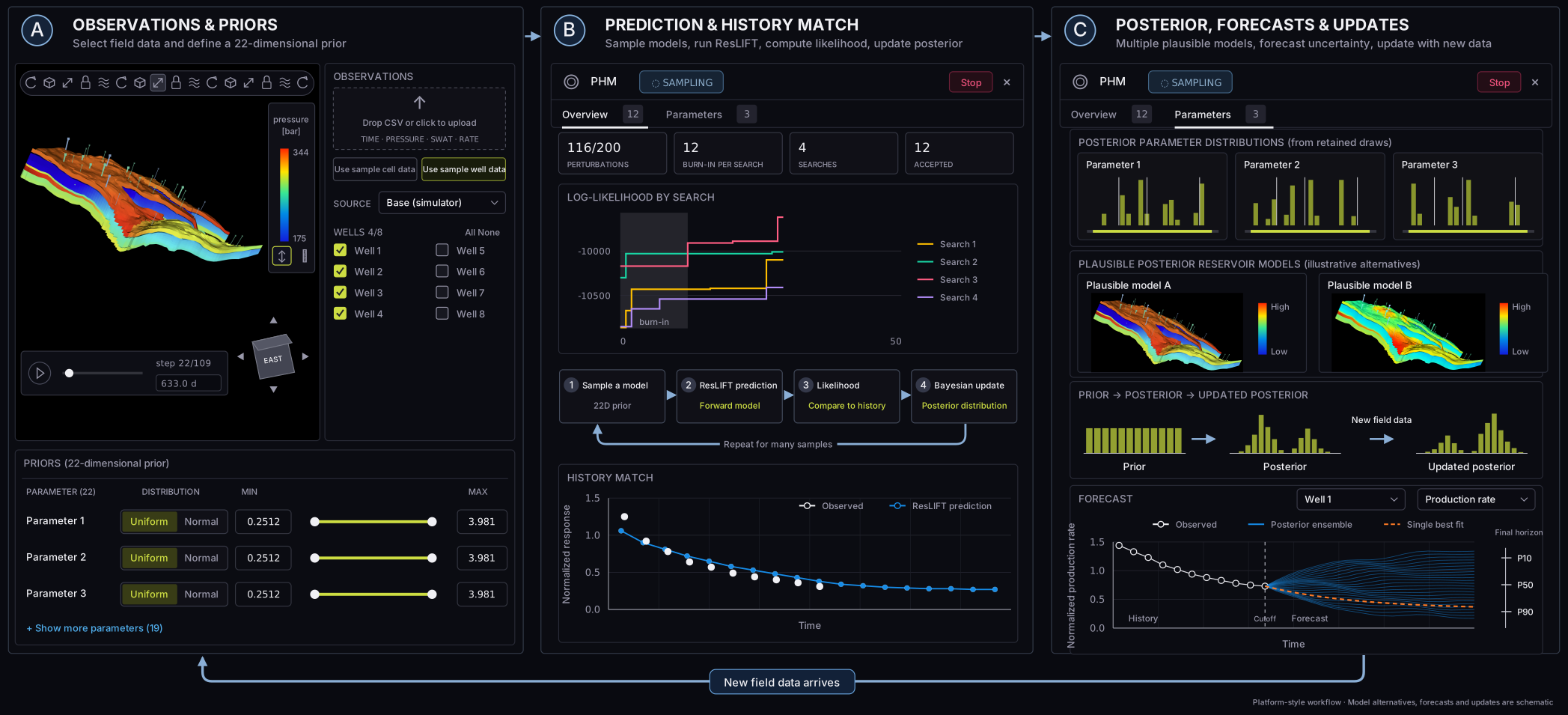
1 From observed history to all plausible models

Let $u$ denote the uncertain reservoir parameters and $d$ the observed history. Bayesian inference combines the prior $p\left(u\right)$, which defines plausible parameter values before seeing the history, with the likelihood $p\left(d\right|u)$, which scores agreement between model predictions and observations. Bayes' rule gives

$$p\left(u\right|d)\propto p(d\left|u\right)p\left(u\right).$$

The posterior $p\left(u\right|d)$ describes parameter uncertainty after conditioning on the observations. An optimizer returns one point, such as the maximum a posteriori model, whereas MCMC draws samples that characterize the full posterior. This distinction matters when several separated regions are plausible. One best-fitting model cannot represent those alternatives, and an average between them may fit the observed history worse than any of them.

2 ResLIFT enables fast discovery of the posterior

Bayes' rule gives the relative posterior support of a proposed reservoir model, but characterizing the distribution requires exploring a continuous parameter space. A grid with $n$ values for each of $m$ parameters requires $n^m$ forward evaluations and quickly becomes impractical. MCMC avoids this exhaustive search by proposing a complete reservoir model, predicting its observations, evaluating its likelihood, and accepting or rejecting it using a posterior-density ratio. The retained states form posterior samples, concentrating computation in regions supported by the prior and observations.

Forward prediction remains the bottleneck because every proposal must be evaluated. A conventional reservoir simulator solves multiphase flow through space and time before computing a single likelihood, while a useful posterior estimate can require tens or hundreds of thousands of such evaluations. The cost can be prohibitive even with few uncertain parameters because sampling error, autocorrelation, and convergence determine the required chain length.

ResLIFT, our reservoir Latent Interaction Field Transformer, is designed for this repeated evaluation. It takes the initial reservoir state, static rock properties, the well-control schedule, and a requested time, then predicts pressure and phase saturation directly at that time. It does not roll through preceding time steps or feed predicted states back into subsequent predictions. The likelihood can therefore query only the times at which observations exist, avoiding unobserved intermediate states and accumulated rollout error. Pressure and saturation can be compared with measurements directly, while responses such as well production rates are derived from the predicted states. Each evaluation takes only a few seconds and replaces the simulator output without changing the Bayesian formulation, making high-dimensional posterior sampling practical.

3 A controlled 22-dimensional Norne benchmark

We present the method on the public Norne black-oil benchmark [1][2]. The uncertain parameter vector $u=(u_1,\dots ,u_{22})$ contains one value for each geological layer. Each $u_k$ is a logarithmic multiplier on the vertical permeability of layer $k$, with a physical multiplier of ${10}^{u_k}$. The parameters have independent priors and are sampled together, so no layer is forced to follow another.

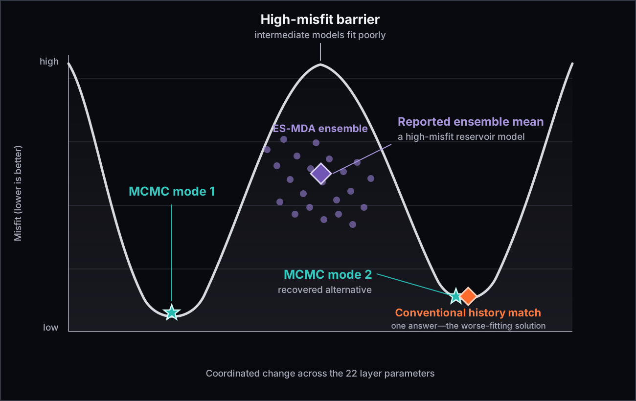
We designed a sparse saturation history to create a controlled multimodal inverse problem. The observations come from one reference reservoir configuration, making that configuration the most accurate match by construction. A second, separated configuration gives a slightly less accurate but still plausible match, while configurations between them disagree much more strongly with the observations. The result is two data-supported regions separated by a low-likelihood barrier, without making the two solutions artificially equal, as illustrated in Figure 2. In this comparison, conventional history matching terminates at the worse-fitting solution and ES-MDA concentrates between the two solutions, whereas MCMC recovers both data-supported modes.

The sampler is not told where either solution lies. It starts from the full prior and explores the complete 22-dimensional space, with every layer free to move independently. Recovering both regions therefore requires discovering coordinated combinations of layer permeabilities; it cannot be achieved by sweeping one global multiplier along a predefined path.

4 Crossing barriers with parallel tempering

The separated plausible regions shown in Figure 2 create a sampling challenge. Standard MCMC can explore a solution once it enters its basin, but moving to the other solution requires crossing models that disagree strongly with the observations. Those moves are rarely accepted, so a longer run can simply produce more samples from the same basin. To discover both solutions without telling the sampler where they are, sampler should be able to cross the high barrier effectively and regularly.

Parallel tempering provides that mechanism by running several MCMC chains at different inverse temperatures, $\beta$ [3]. At each value of $\beta$, MCMC targets a tempered posterior

$${\pi }_{\beta }(u)\propto p(u){p(d|u)}^{\beta }.$$

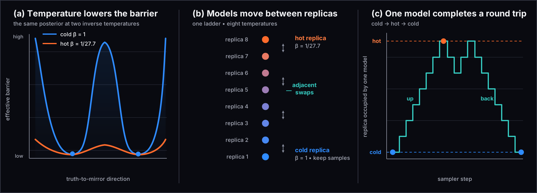
At the coldest chain, $\beta =1$, the likelihood is unchanged and the chain samples the posterior. Decreasing $\beta$ weakens the influence of the likelihood and flattens the barrier between the two solutions. As $\beta$ approaches zero, the tempered posterior approaches the prior.

Each temperature-specific chain is called a replica, and the ordered set of replicas forms a temperature ladder. Neighboring replicas periodically exchange their complete 22-layer reservoir models. A model can move up the ladder, cross the barrier in a warmer replica, and return to the cold replica in the other basin. This lets the sampler discover both explanations without distorting the posterior. Only samples from the cold replica are retained for inference. The parallel tempering mechanism is illustrated in Figure 3.

5 What the observations can and cannot identify

Probabilistic history matching does not force every uncertain parameter toward a single answer. It shows how strongly the observations constrain each parameter and where different parameter combinations produce nearly the same observed history. A parameter is identifiable only if the observations can distinguish its effect while the other uncertain parameters are allowed to vary. In the posterior, a marginal distribution that contracts relative to its prior indicates that the data have constrained that parameter. A marginal that remains close to the prior indicates weak information, while separated regions of posterior support distinct parameter combinations that remain consistent with the observations.

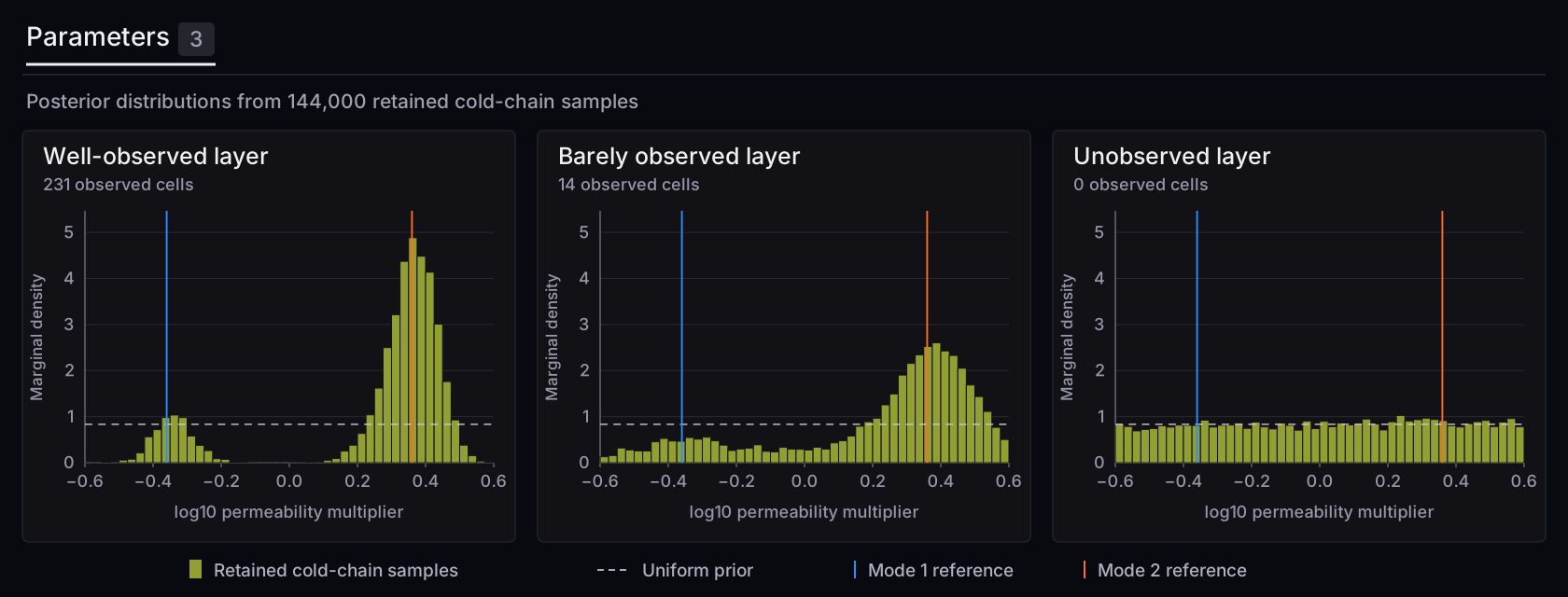
The 22 layer-permeability multipliers benchmark illustrates this distinction. Selected observables strongly constrain a well-observed layer while retaining the two modes created for this benchmark. A barely observed layer is only weakly constrained, so its posterior remains much broader. For a layer with no observations, the posterior stays close to the prior. This is not a failure. It is the method correctly reporting that the history does not identify that parameter. These three cases are compared in Figure 4.

This distinction changes how field data should be collected. The most useful next observation is not simply another measurement where the models already agree. It is one taken in a location or at a time where the remaining reservoir explanations predict different outcomes. Posterior uncertainty can therefore guide the choice of observable, sensor location, and sampling time toward parameters that are both decision-relevant and still poorly identified.

6 From history matching to better forecasting

The value of probabilistic history matching lies in replacing a single calibrated realization with a posterior distribution over models that remain plausible given the observations and prior knowledge. This value does not depend on the posterior having multiple modes. The distribution may concentrate around one region, remain broad, or contain several separated regions. Each outcome reveals something different about what the observed history has resolved.

ResLIFT makes it practical to explore these alternatives instead of stopping at the model found by an optimizer. Posterior samples can be propagated through future operating scenarios to turn uncertainty in reservoir properties into uncertainty in production forecasts. Development plans can then be compared by how they perform across the plausible reservoir models, not only under a single best fit.

The posterior also provides a map for collecting better data. Where plausible models make nearly identical predictions, another measurement adds little information. Where their predictions diverge, a targeted observation can distinguish between them and reduce uncertainty that matters to the forecast. As new field data arrive, they can be assimilated to update the posterior and sharpen the next round of forecasts and measurement choices.

A useful history match should clarify both what has been learned and what remains uncertain. Probabilistic history matching preserves uncertainty where the data cannot resolve it and reduces it where they can. The result is a set of forecasts and decisions that can be traced back to the observations rather than a single answer that conceals the alternatives.

References

1. Statoil. (2018). Benchmark case Norne. Zenodo. https://doi.org/10.5281/zenodo.1213195.
2. Open Porous Media Initiative. (n.d.). Open datasets: Norne. https://opm-project.org/?page_id=559.
3. Earl, D. J., and Deem, M. W. (2005). Parallel tempering: Theory, applications, and new perspectives. Physical Chemistry Chemical Physics, 7, 3910–3916. https://doi.org/10.1039/B509983H.