Turn terabytes of simulation results into a portable model of reservoir behavior. Explore more possible futures, then bring that intelligence closer to the asset.
An infill well can look attractive in one reservoir realization and disappoint in another. Fault communication, permeability and fluid contacts change where the remaining oil sits, how pressure responds and when water arrives. A development decision needs those alternatives on the table while there is still time to act.
Yet exploring them can become a months-long exercise in terminal sessions, input-deck edits, script maintenance, job launches, crash diagnosis and processing tens of terabytes of results. Across an asset's life, simulation knowledge accumulates faster than teams can reuse it. The practical cost is a narrower set of questions investigated before the next decision.
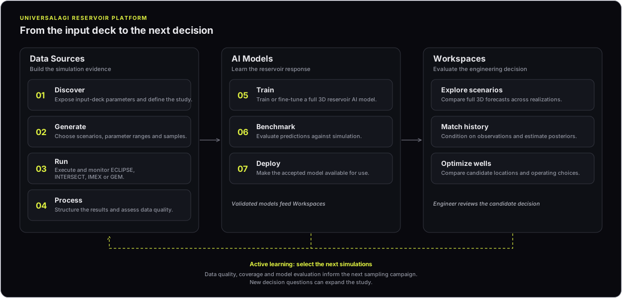
UniversalAGI Reservoir Platform puts full 3D AI models at the center of reservoir engineering. Simulation provides the physical evidence for training and evaluation. The platform turns that evidence into reusable models that power scenario exploration, history matching and well optimization. Engineers define the physical assumptions and decision criteria; the platform manages the data and model lifecycle. Figure 1 shows how the three parts of the platform connect.
1 Data Sources: make each simulation part of a larger study
A useful AI model begins with the uncertainties the engineer needs to investigate. Data Sources is designed to expose the full input-deck parameter space, including equilibrium regions, permeability, porosity, fault transmissibility multipliers, PVT tables, and well specifications and controls. Each study selects the parameters to vary; scenario templates turn those choices into a repeatable sampling campaign.
For a formation-factor or water-breakthrough scenario, the engineer selects parameter ranges and generates realizations. The platform coordinates and monitors simulation campaigns using ECLIPSE, INTERSECT, IMEX or GEM. Sample coverage and job status are visible together, so missing results and failed jobs can be traced back to the study design. Figures 2a to 2d show the study design, run monitoring, result inspection and scenario selection views.
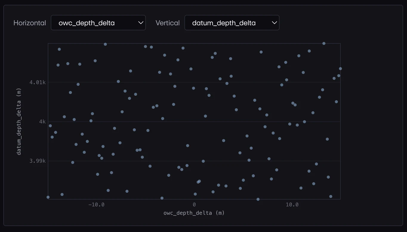
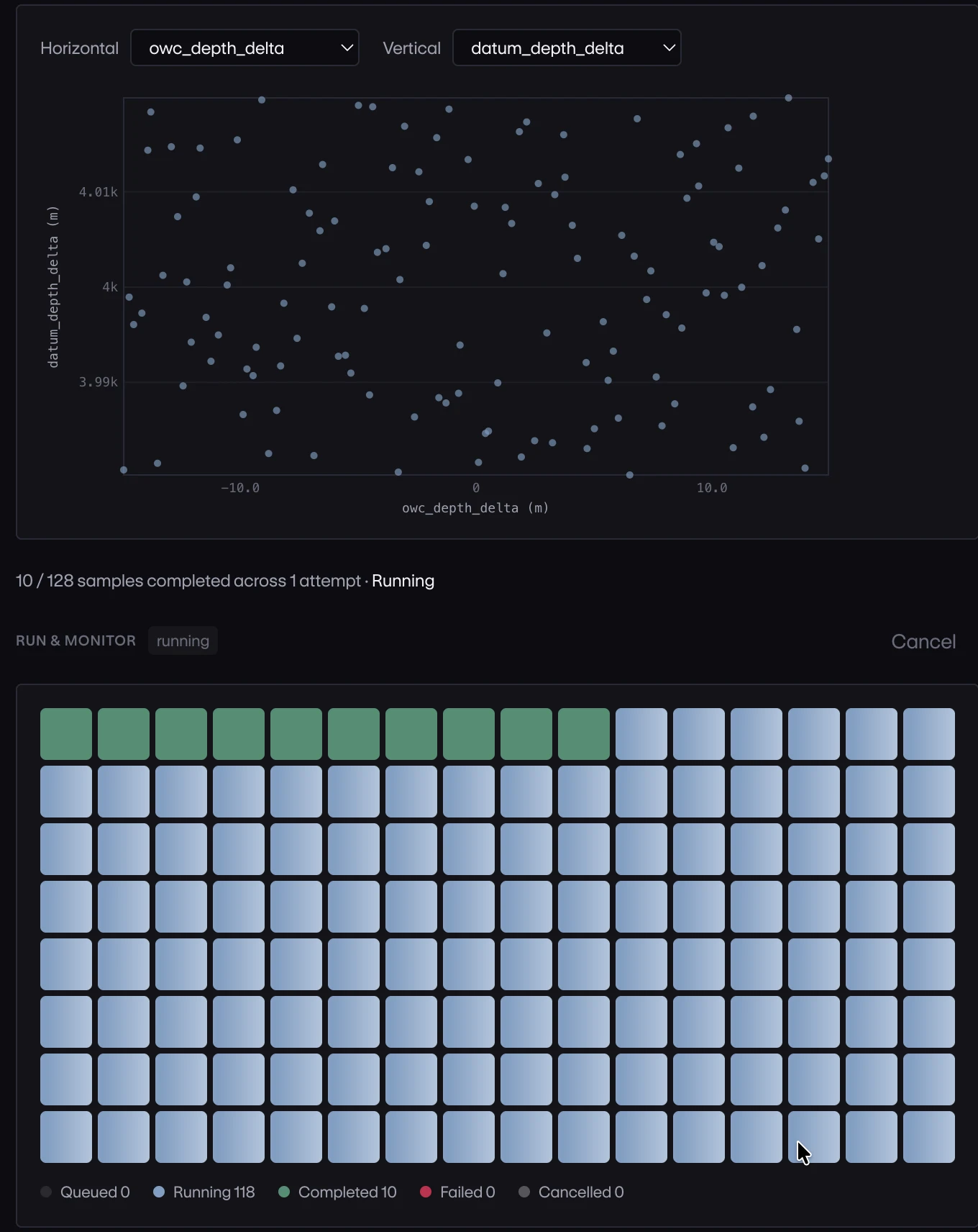
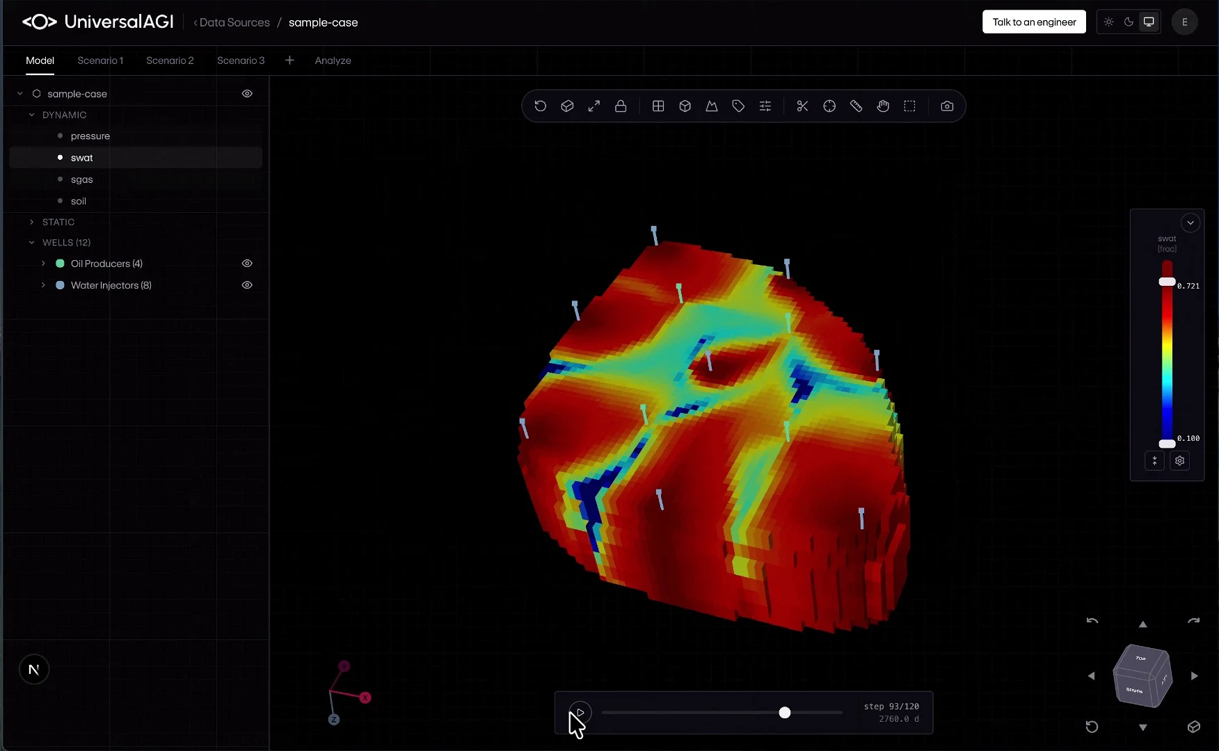
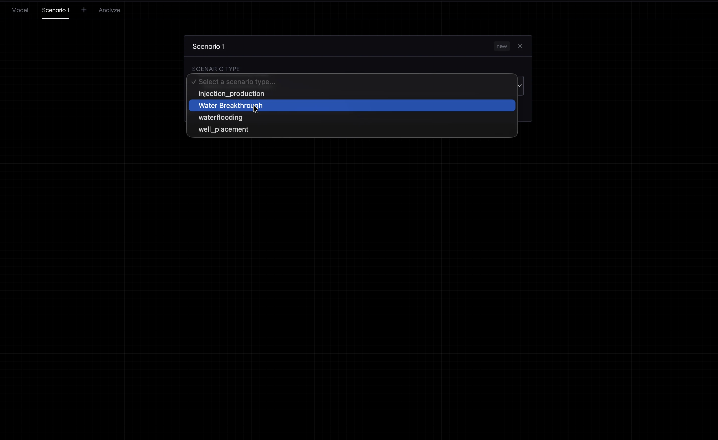
Results become structured datasets with quality reports that guide the next iteration. Engineers can inspect pressure and saturation fields through time, review the quality of the data and identify gaps before training. Active learning helps select additional simulations where new evidence is most useful to the next phase.
This changes how simulation budgets are spent: broad initial coverage can be followed by targeted investigation of the uncertainties that matter to the decision.
2 AI Models: put full 3D prediction in the engineer's hands
AI Models turns a simulation dataset into a reusable approximation of reservoir behavior. Ready-to-use templates bring modern reservoir physics model architectures into a workflow that requires no training code. Engineers choose the source case, scenarios and model configuration. The interface includes LIFT and XMeshGraphNet architectures and separates training, validation and test realizations, as shown in Figure 3.
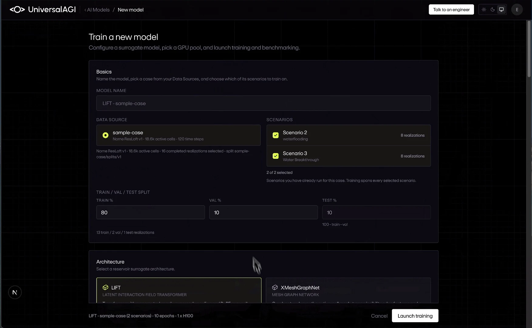
The model is parameterized on the physical inputs configured for the study: reservoir properties, initial conditions and well controls become pressure and phase-saturation trajectories throughout the 3D grid. Model selection and evaluation serve the downstream task, including history matching, well optimization and probabilistic inference. Reusing the learned mapping makes their repeated forward evaluations affordable.
Carry the learned response, without moving the archive
A multi-million-parameter model can encode relationships learned from terabytes of simulations in weights small enough for laptop memory. For scale, 50 million parameters stored at 32-bit precision occupy 200 MB. This is illustrative weight storage, not a measured UniversalAGI model size. Geometry, inputs, intermediate activations and generated fields add to the inference memory budget.
The compact model approximates the reservoir's response within its learned domain. Original results remain available centrally for traceability, retraining and detailed checks. Engineers carry the predictive model and the inputs for their investigation.
Training management and quality reports show where predictions agree with simulation and where errors grow. Acceptance needs checks on full forecast trajectories, water-front arrival and well response; average error alone can hide local failures. Deployment makes the accepted model available for use within its evaluated conditions. The simulator remains the physical reference.
3 Workspaces: make the next reservoir decision with more evidence
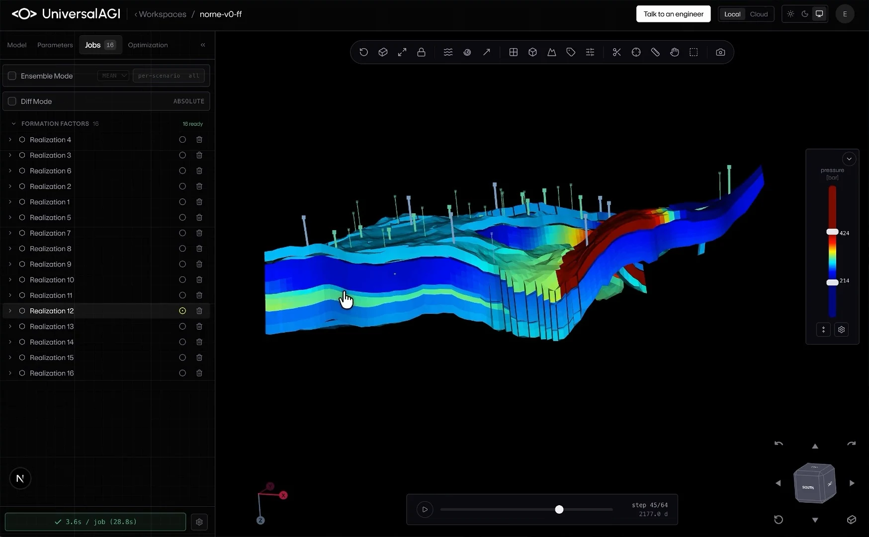
Workspaces puts the trained model inside the engineer's daily investigation. Change the selected parameters, generate alternative realizations, and inspect pressure and fluid saturations across the 3D reservoir through time. Individual cells connect to response curves, so a difference in forecast can be traced to where and when it develops.
The performance ambition
Our performance goals are thousands of scenario evaluations in seconds for work that can otherwise occupy hours to days; history matching and well optimization in minutes within studies that can take weeks to months; and full 3D probabilistic history matching and posterior estimation in hours. These goals assume a suitable trained model and compute configuration, excluding simulation-data generation and training. Study duration and inference runtime measure different parts of the workflow; the examples below report individual runs, not matched speedup benchmarks.
Explore the alternatives behind a forecast
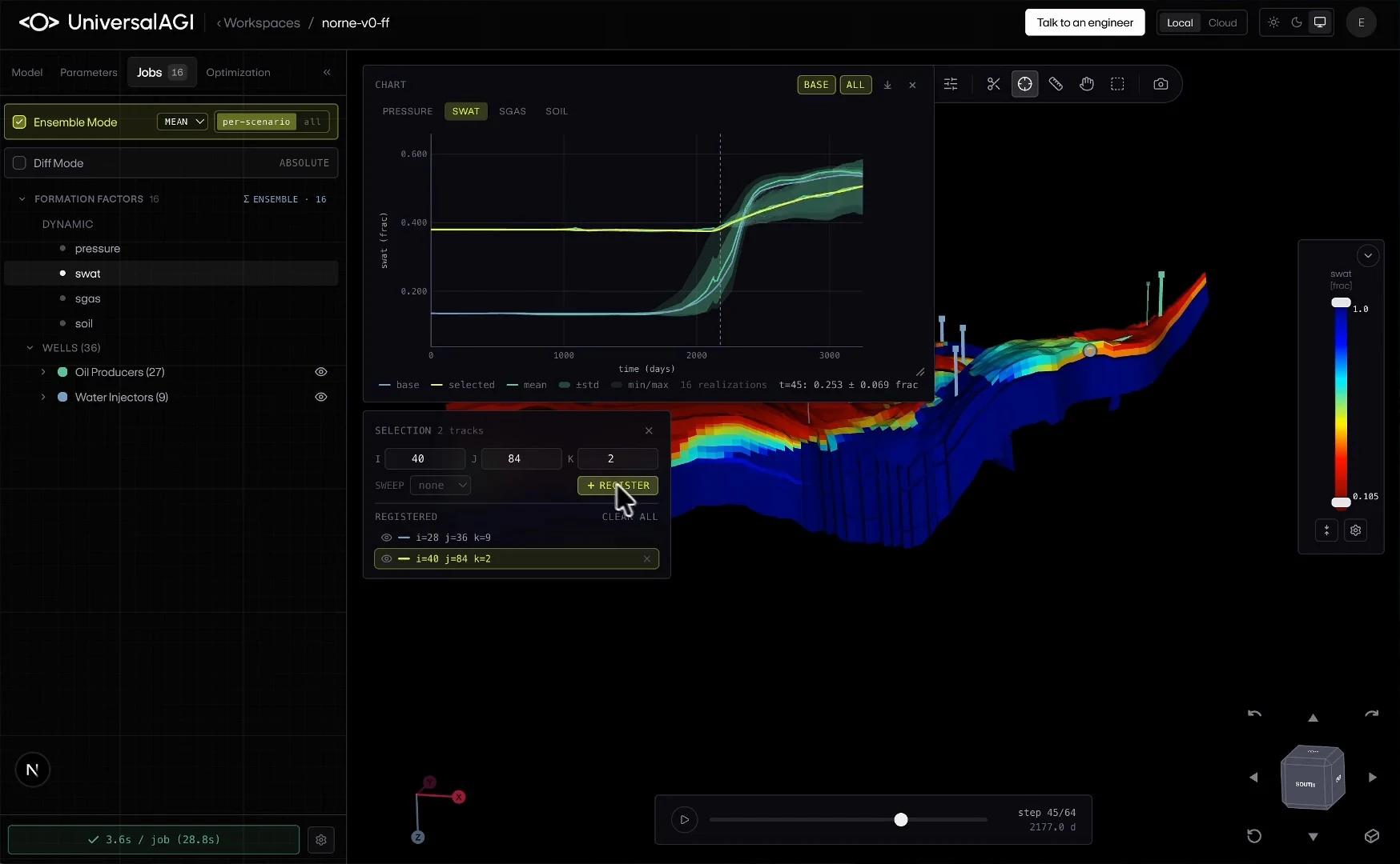
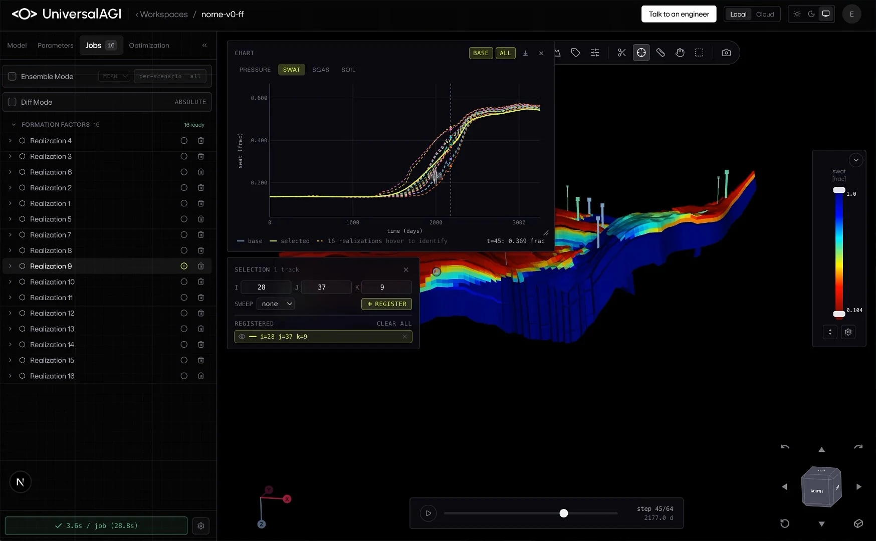
The ensemble view in Figure 4a already compares water-saturation trajectories across 16 realizations. The broader vision is an interactive workspace holding hundreds of alternative reservoir descriptions, sharing one trained model and generating forecasts on demand. The objective is to make ensemble investigation practical on local hardware by reducing repeated solver work and movement of simulation archives.
In this design, realizations are evaluated in batches, updating the mean, standard deviation, minimum and maximum as results arrive. These statistics can be accumulated without retaining every trajectory. Selected forecasts can be retained for 3D inspection; full ensemble outputs need their own storage budget. For illustration, 500 realizations of 100,000 cells, 64 times and four FP32 fields occupy 51.2 GB before metadata.
At each cell and time, the mean describes the ensemble response, standard deviation its dispersion, and minimum/maximum the sampled lower and upper envelope. These extrema bound the selected samples; calibrated uncertainty or posterior intervals require additional assumptions and evaluation.
Match observations and inspect the fit
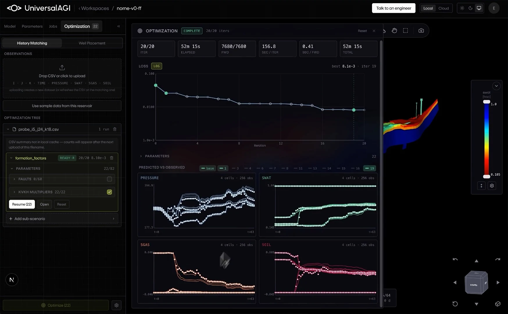
History matching brings observations into the loop. The Norne run in Figure 5 adjusts 22 selected permeability-ratio multipliers and completes 7,680 forward evaluations over 20 iterations in 52 minutes 15 seconds. The workspace shows convergence alongside predicted and observed pressure, water saturation, gas saturation and oil saturation. Engineers can review the fit before accepting a candidate reservoir description.
Compare well locations before committing
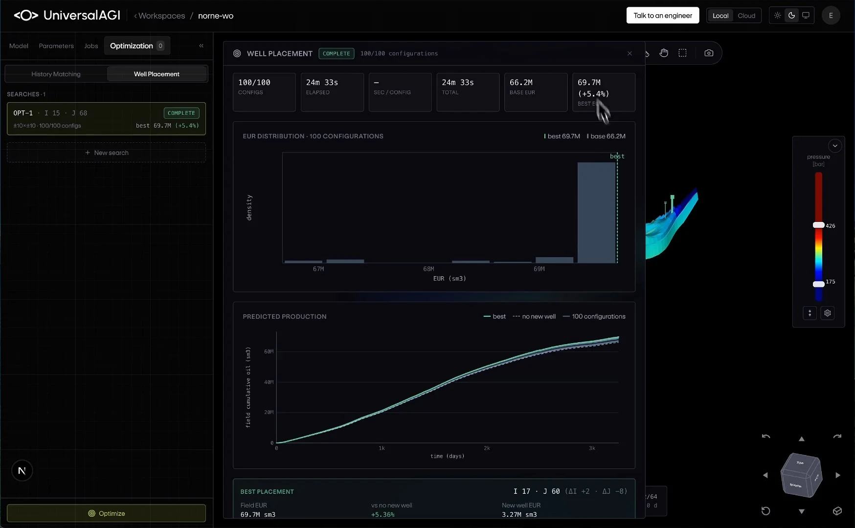
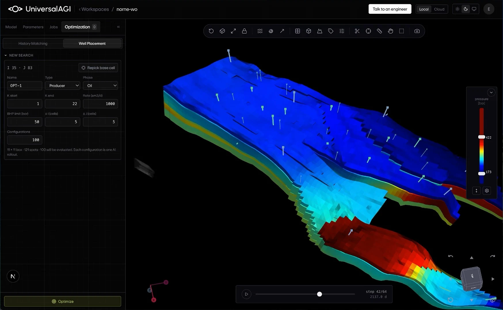
For well placement, the engineer specifies the well type, completion interval, rate and pressure limits, and search area. The search in Figure 6a evaluates 100 configurations in 24 minutes 33 seconds. Its best candidate reaches a predicted field estimated ultimate recovery (EUR) of 69.7 million standard cubic metres, against a 66.2 million baseline without the new well. The interface reports a 5.4% increase in predicted EUR for this case.
The useful output is a set of candidate locations with production forecasts and a visible comparison to the baseline. Engineers can take the preferred candidates forward for simulator confirmation and economic assessment. Figure 6b shows how a search is defined in the reservoir view.
Carry uncertainty into the decision
Workspaces also supports probabilistic history matching and posterior estimation, using full 3D AI predictions to evaluate reservoir parameters conditioned on observations. The engineering value is a range of credible forecasts against which to assess a development choice. Observation uncertainty, the geological prior and model error all affect the resulting posterior; the ensemble plot in Figure 4a illustrates scenario spread.
4 Across the life of the asset: make every valid realization teach the model
The goal is a persistent asset record in which every valid simulation remains available for learning, evaluation and future decisions. A study's preferred outcome does not decide which data survives.
A fault assumption later rejected for the asset can still teach a useful conditional response, provided that assumption is represented in the model inputs and the simulation is physically consistent. History matching changes which realizations are credible for the asset; it need not erase their value as training examples.
Diverse geology and operating conditions can expand generalization when coverage, sampling balance and held-out evaluations improve together. Incorrect physics or corrupted outputs teach errors. The longer-term opportunity is pretraining across studies and adapting to new assets, consistent with the transfer-learning direction demonstrated by PDE foundation models such as Poseidon. Asset-specific forecast evaluation remains necessary.
5 The next horizon: a reservoir twin that works alongside the asset
Our vision is to deploy the learned reservoir response near the asset, connected to measurements and a supervisory controller. Pressure, production rates and water cut update estimates of reservoir state and the probabilities of alternative realizations. Local inference evaluates what could happen under the next operating choices. That continuing connection to the physical asset makes the model part of a digital twin.
Training and large simulation campaigns remain on central compute. A versioned inference package runs on an appropriately sized asset-side workstation or edge server, following the training-to-edge pattern already used in industrial AI. Measurements update the estimated state and realization probabilities during operation; new model weights arrive through separately evaluated releases.
Future architecture: observe, predict, decide, update
- Observe. Assimilate measurements into the state and reservoir ensemble.
- Predict. Forecast candidate controls across the conditioned ensemble.
- Decide. Compare value and downside risk under operating constraints.
- Update. Apply the authorized control step; measure and plan again.
Simulation and training supply evaluated model releases. Asset measurements close the operating loop. This is the proposed architecture beyond the workspace examples shown above.
A model-predictive controller would search injection and production schedules across the conditioned ensemble, balancing expected recovery or economic value against downside risk while enforcing specified well-pressure, rate and facility constraints in its predictions. It applies the first authorized step, then replans as measurements arrive. Learned predictive-control research makes constraint handling and closed-loop behavior central to this design.
The operating cadence must match reservoir response, observation quality and available compute. Fast equipment and safety controls continue independently; unfamiliar conditions trigger simulator review and targeted new training data. The destination is an asset that carries its accumulated simulation knowledge into each operating decision, with engineers setting objectives and authority.
Interface examples show Norne and sample-case demonstrations from UniversalAGI. Timings refer to the displayed runs and depend on the model, workload and compute configuration.